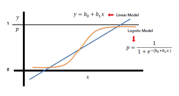
The logit model is a modification of linear regression that makes sure to output a probability between 0 and 1 ( classification with two classes) by applying the sigmoid function,which, when graphed, looks like the characteristic S-shaped curve.


In logistic regression, the cost function is basically a measure of how often you predicted 1 when the true answer was 0, or vice versa. Below is a regularized cost function just like the one we went over for linear regression.

The first chunk is the data loss, i.e. how much discrepancy there is between the model’s predictions and reality. The second chunk is the regularization loss, i.e. how much we penalize the model for having large parameters that heavily weight certain features (remember, this prevents overfitting). We’ll minimize this cost function with gradient descent, as above, and voilà! we’ve built a logistic regression model to make class predictions as accurately as possible.

- True Positive = TP = positivt predictade värden som verkligen är positiva
- True Negative = TN = negativt predictade värden som verkligen är negativa
- False Positives = FP = Type I error = positivt predictade värden som verkligen är negativa
- False Negatives = FN = Type II error = negativt predictade värden som verkligen är positiva
- Simple baseline = TN+FP / Alla värden
- Accuracy = TP + TN / Alla värden
- Sensitivity = True Positive rate TP/(TP+FN)= andelen positiva fall vi har klassiferat rätt
- Specificity = True Negative rate TN/(TN+FP) = andelen negativa fall vi har klassiferat rätt
- Fall-out = False Positive rate FP/(FP+TN)

R:
- Null deviance : when only using the intercept
- Residual deviance : include all the variables
- AIC like adj R^2 skall helst vara lite. can only be compared between models on the same data set
table(qualityTrain$PoorCare, predictTrain > 0.7)
- library(broom)
- model %>% augment(type.predict = “response”)
- augment(mod, type.predict = “response”) %>% mutate(pred = round(.fitted))
- augment(mod, newdata = new_data, type.predict = “response”)
-
- data_space <- ggplot(data = MedGPA_binned, aes(x = mean_GPA, y = acceptance_rate)) +
geom_point() + geom_line() - MedGPA_plus <- mod %>% augment(type.predict = “response”)
- data_space + geom_line(data = MedGPA_plus, aes(x = GPA, y = .fitted), color = “red”)
- data_space <- ggplot(data = MedGPA_binned, aes(x = mean_GPA, y = acceptance_rate)) +
- mutate(log_odds = log(acceptance_rate / (1 – acceptance_rate)))
- mutate(log_odds_hat = log(.fitted / (1 – .fitted)))
ROCRpred = prediction(predictTrain, qualityTrain$PoorCare)
ROCRperf = performance(ROCRpred, “tpr”, “fpr”)
ROCRperfTest = performance(ROCRpredTest, “tpr”, “fpr”)
auc = as.numeric(performance(ROCRpredTest, “auc”)@y.values)
auc
# draw 3D scatterplot
p <- plot_ly(data = nyc, z = ~Price, x = ~Food, y = ~Service, opacity = 0.6) %>% add_markers()
# draw a plane
p %>% add_surface(x = ~x, y = ~y, z = ~plane, showscale = FALSE)
P:
from sklearn.linear_model import LogisticRegression
#Assumed you have, X (predictor) and Y (target) for training data set and x_test(predictor) of test_dataset
# Create logistic regression object
model = LogisticRegression()
# Train the model using the training sets and check score
model.fit(X, y)
model.score(X, y)
#Equation coefficient and Intercept
print(‘Coefficient: \n’, model.coef_)
print(‘Intercept: \n’, model.intercept_)
#Predict Output
predicted= model.predict(x_test)