Principal Component Analysis (PCA)
Dimensionality reduction looks a lot like compression. This is about trying to reduce the complexity of the data while keeping as much of the relevant structure as possible
Cucumbers and iceberg lettuce contain of 96% water
- A technique used to emphasize variation and bring out strong patterns in a dataset
- Often used to make data easy to explore and visualize
- Compressing data in some meaning-preserving way before feeding it to a deep neural net or another supervised learning algorithm.
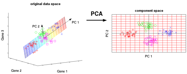
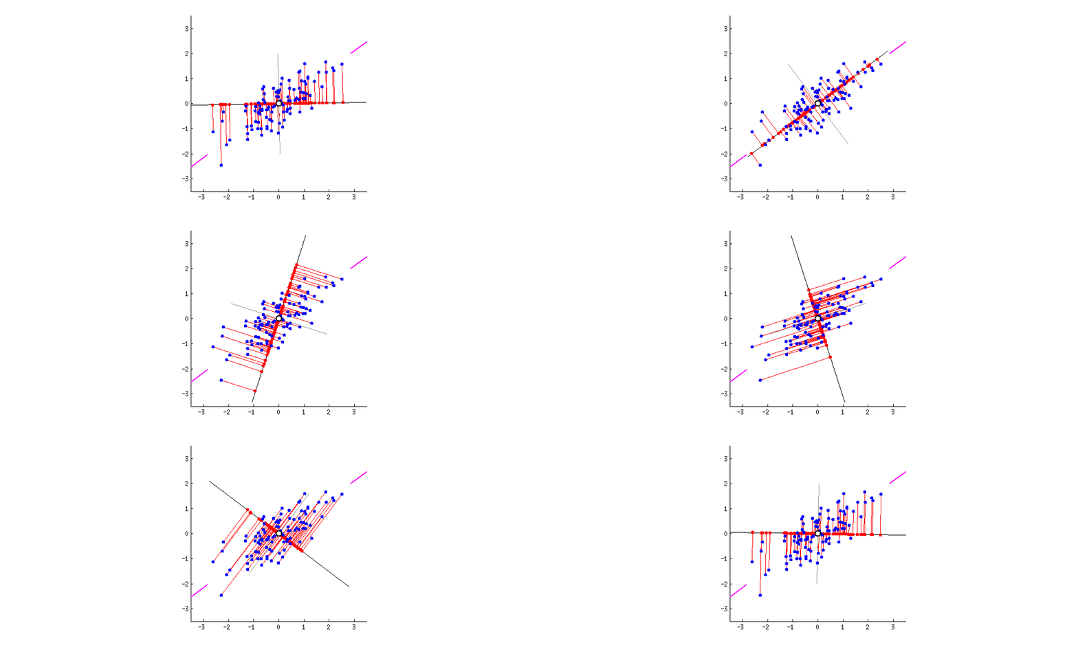
Come up with a basis for the space and then select only the most significant vectors that explain most of the space. These basis vectors are called principal components and the subset you select constitute a new space that is smaller in dimensionality than the original space but maintains as much of the complexity of the data as possible. To select the most significant principal components, we look at how much of the data’s variance they capture and order them by that metric.
Transformed dimension
The transformation definition makes sure that the principal components are ordered by variance so that by making use of the first several dimensions only, we can start gaining an understanding of the dataset’s organization.
http://setosa.io/ev/principal-component-analysis/


R: